Gene maps can be created by using the information obtained through a series of test crosses, whereby one of the parents is heterozygous for a different pair of genes and we can calculate the recombination frequencies between pairs of genes. A test cross between two genes is called a two-point test cross. Let us explore a worked example which will demonstrate how we are able to gene map using recombination frequencies. First, we will look at two-point test crosses, then we will investigate three-point test crosses, which are generally more accurate.
A scientist conducted a sequence of two-point crosses for four genes, q, r, s and t, and the following recombination frequencies were obtained, as shown in Ta
Table 11.3.1 Recombination Frequencies for a Sequence of Two-Point Crosses for Four Genes (q, r, s & t) | Gene loci | RF (%) |
|---|
| q and r | 50 |
| q and s | 50 |
| q and t | 50 |
| r and s | 20 |
| r and t | 10 |
When independent assortment is occurring, we have RF = 50%. So, we can deduce that genes q and r are either located on different chromosomes or are very distant from each other on the same chromosome. They are hence considered to belong to different linkage groups. By the same virtue, q and s are also in different linkage groups, as are q and t. Now, the RF between r and s is 20%, so these genes are separated by 20 map units. Genes r and t are also linked, with an RF of 10%. To determine if gene t is 10 m.u. to the right or left of gene r, we look at the  distance. If t is 10 m.u. to the left of r, then the distance between t and s should be approximately the sum of the distance between r and s and between s and t:
 ") . [Note: this distance is an approximation due to “double crossovers” occurring]. Now, the other possibility is that gene t is located to the right of gene r, and in that case, the distance between gene t and s will be less
. [Note: this distance is an approximation due to “double crossovers” occurring]. Now, the other possibility is that gene t is located to the right of gene r, and in that case, the distance between gene t and s will be less  . We see from the data that the R.F. between s and t is 28%, so the t lies to the left of r. So, we can draw the genetic map as shown in Figure 11.3.1.

Figure 11.3.1 Genetic Map Based on Data Obtained From Two-Point Crosses in
Table 11.3.1. [
Long description]
Watch the following video, Genetic Distance and Two-Point Mapping, by Joseph Ross (2017) on YouTube.
One or more interactive elements has been excluded from this version of the text. You can view them online here: https://opengenetics.pressbooks.tru.ca/?p=1056#oembed-1
Next, take a look at the video below, Gene Mapping, Percent Recombination and Map Units, by AK Lectures (2015) on YouTube, for another worked example of gene mapping using % recombination.
One or more interactive elements has been excluded from this version of the text. You can view them online here: https://opengenetics.pressbooks.tru.ca/?p=1056#oembed-2
We see that a two-point test cross is a method to estimate gene distances in map units using recombination frequency data. We also mentioned that the occurrence of double crossovers causes an underestimation of map distances. Generally, the larger the recombinant frequency, the less accurate it is as a measure of map distance. In fact, map units calculated from larger recombinant frequencies are actually smaller than map units calculated from smaller recombinant frequencies. Typically, when measuring recombination between three linked loci, the sum of the two internal recombinant frequencies is greater than the recombinant frequency between the outside loci. The best estimates of map distance are obtained from the sum of the distances calculated for shorter sub-intervals. Refer to Figure 11.2.3 which demonstrates “a double crossover” and shows only the middle gene being altered in such cases, vs. the results with single crossovers. A genetic map consists of multiple loci distributed along a chromosome. A particularly efficient method of mapping three genes at once is the three-point cross, which allows the order and distance between three potentially linked genes to be determined in a single cross experiment (Figure 11.3.2).
/07%3A_Linkage_and_Mapping/7.07%3A__Mapping_With_Three-Point_Crosses")
Figure 11.3.2 A Three-Point Cross for Loci Affecting Tail Length, Fur Colour, and Whisker Length [
Long description]
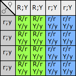
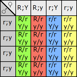
This is particularly useful when mapping a new mutation for which the location is unknown relative to two previously mapped loci with known locations. The basic strategy is the same as for the dihybrid mapping experiment described previously, except pure breeding lines with contrasting genotypes are crossed to produce an individual heterozygous at three loci (a trihybrid), which is then test-crossed to a tester, which is homozygous recessive for all three genes, to determine the recombination frequency between each pair of genes, among the three loci. A Punnett square can be used to predict all the possible outcomes of the test cross (Figure 11.3.3). The progeny produced from the test cross is shown in Table 11.3.2.

Figure 11.3.3 Punnett Square of the Test Cross for
Figure 11.3.2, Showing the Predicted Gametes Possible from this Cross, and the Resulting Phenotypes [
Long description]
Table 11.3.2 An Example of Data that Might be Obtained from the F2 Generation of the Three-Point Cross is Shown in Figure 11.3.2. The rarest phenotypic classes correspond to double recombinant gametes ABc and abC. Each phenotypic class and corresponding gamete can also be classified as parental (P) or recombinant (R) with respect to how each pair of loci (A,B), (A,C), (B,C) are arranged on the chromosome. | tail phenotype | fur phenotype | whisker phenotype | number of progeny n=120 | gamete from trihybrid | genotype of F2 from test cross | loci A, B | loci A, C | loci B, C |
|---|
| short | brown | long | 5 | aBC | aaBbCc | P | R | R |
| long | white | long | 38 | AbC (P2) | AabbCc | P | P | P |
| short | white | long | 1 | abC | aabbCc | R | R | P |
| long | brown | long | 16 | ABC | AaBbCc | R | P | R |
| short | brown | short | 42 | aBc (P1) | aaBbcc | P | P | P |
| long | white | short | 5 | Abc | Aabbcc | P | R | R |
| short | white | short | 12 | abc | aabbcc | R | P | R |
| long | brown | short | 1 | ABc | AaBbcc | R | R | P |
When the trihybrid is crossed to a tester, it should be able to make eight different gametes, to make eight possible different phenotype combinations in the offspring. The next step would be to identify if the alleles are recombinant or parental gametes. This can be done by comparing only two loci at one time to the parental gametes. In this example, the parents of the trihybrid are a/a B/B c/c, and A/A b/b C/C, so the parental gametes would be aBc and AbC respectively. Now, by comparing two loci at once you can determine if, between the two, they are recombinant or parental. For example, the offspring in the first row in Table 11.3.2 came from gamete aBC. Comparing loci A and B, we see that it matches one of the parental gametes and, therefore, it is parental. Comparing A and C, we see that it matches neither parental — so it is recombinant. The same can be said for comparing B and C.
}{120}=\frac{30}{120}=25\%")
}{120}=\frac{12}{120}=10\%")
}{120}=\frac{38}{120}=32\%") [not corrected for double crossovers]
[not corrected for double crossovers]
Once the classes of progeny have been identified, as each pair of locus being parental or recombinant, recombination frequencies may be calculated for each pair of loci individually — as we did before for one pair of loci in our dihybrid cross (Chapter 18). We can then use these numbers to build the map, placing the loci with the largest RF on the ends. However, note that in the three-point cross, the sum of the distances between A-B and A-C (10% + 25% = 35%) is less than the distance calculated for B-C (32%). This is because of double crossovers between B and C, which were undetected when we considered only pairwise data for B and C (Figure 11.3.4). We can easily account for some of these double crossovers, and include them in calculating the map distance between B and C, as follows.


Figure 11.3.4 Two Possible Maps Based on the Data in
Table 11.3.2 (Without Correction for Double Crossovers) [
Long description]
We already deduced that the map order must be BAC (or CAB). However, these double recombinants, ABc and abC, were not included in our calculations of recombination frequency between loci B and C. If we included these double recombinant classes (multiplied by 2, since they each represent two recombination events), the calculation of recombination frequency between B and C is as follows, and the result is now more consistent with the sum of map distances between A-B and A-C.
+2(1))}{120}=\frac{42}{120}=35\%") [corrected for double crossovers]
[corrected for double crossovers]
As such, the three-point cross is useful for:
- determining the order of three loci relative to each other,
- calculating map distances between the loci, and
- detecting some of the double crossover events that would otherwise lead to an underestimation of map distance.
However, it is possible that other, double crossovers events remain undetected, for example double crossovers between loci A&B or between loci A&C. Geneticists have developed a variety of mathematical procedures to try to correct for such double crossovers during large-scale mapping experiments. As more and more genes are mapped, a better genetic map can be constructed. Then, when a new gene is discovered, it can be mapped relative to other genes of known location to determine its location. All that is needed to map a gene is two alleles, a wild type allele and a mutant allele. Now that we know what the map looks like, the frequency of each offspring type can be explained. Parental gametes (AbC and aBc) are the result of no crossovers, or double crossovers between two alleles. Because we know all three loci are linked, it is expected for this frequency to be relatively high, much like what we see in the example above. There are recombinant gametes that are the result of one crossover between two alleles (aBC, Abc, ABC and abc). Single crossover events are more common, but are more likely to happen between loci B and A, because they are 25 cM, and as such, are farther apart than A and C, which are only 10 cM. So, we expect to see more recombinant gametes with the former.
And lastly, there are recombinant gametes that are a result of double crossover events (ABc and abC). Double crossovers between three linked genes like this is rare, so we don’t expect to see many offspring from these recombinant gametes.
The frequencies we see from this cross agree with our expectations. Figure 11.3.6 shows a diagram of the crossover events that took place in regard to recombinant gametes and the number of offspring seen with that gamete type.
In the example given above, all the genes present are linked, with one pair more strongly linked than the other (A and C have stronger linkage than A and B). When choosing three genes to map, this will not always be the case. Sometimes, you will have all genes linked. Sometimes, you may have two genes linked and one gene unlinked. And sometimes, they all may be unlinked (Figure 11.3.5). Much like what we did above, by comparing the ratios of offspring, you should be able to predict if the genes in the trihybrid are linked or not.

Figure 11.3.5 Examples of How Three Genes can be Associated with Each Other, Based on Whether All Three are Unlinked, All Three are Linked, or Two are Linked and One Unlinked [
Long description]
If all three genes are unlinked, then we expect independent assortment and an equal number of all progeny types. Like in the example, if all are linked, you expect there to be many parental genotypes, some recombinant genotypes if they are a result of a single recombination events. Recombinant genotypes that are a result of two recombination events will be rare. The actual numbers of each will differ depending if all the linked genes are equal distances from each other, or if one pair is more linked than the other. In the case where two genes are linked and one gene is unlinked, the following applies. As in the example before, we will use the same parental gametes (AbC and aBc), but will assume the genes A and C are linked and B is unlinked. In this case, because linkage causes a higher prevalence of parental gametes, we expect there to be more parental organizations of A and C, and fewer recombinant organizations of A and C. The presence and/or absence of parental B is not important here, because it is unlinked and will assort independently.

Figure 11.3.6 Diagram of the Crossover Events to Create the Different Recombinant Gametes from the Cross in
Figure 11.3.2. The parental alleles are seen on the black chromosomes. The coloured lines indicate where the crossover event took place, and highlight the alleles for that recombinant gamete. Below each diagram is the recombinant gamete and the number of progeny seen in that cross per
Table 11.3.2. [
Long description]
Take a look at the video, Three-Point Mapping and Gene Order, by Joseph Ross (2017) on YouTube, which gives a worked example of genetic mapping using three-point test crosses.
One or more interactive elements has been excluded from this version of the text. You can view them online here: https://opengenetics.pressbooks.tru.ca/?p=1056#oembed-3
Media Attributions
- Figure 11.3.1 by N. Ramroop Singh
- Figure 11.3.2 Original modified by Deyholos/Locke (2017), CC BY-NC 3.0, Open Genetics Lectures
- Figure 11.3.3 Original by L. Canham (2017), CC BY-NC 3.0, Open Genetics Lectures
- Figure 11.3.4 Original by Deyholos (2017), CC BY-NC 3.0, Open Genetics Lectures
- Figure 11.3.5 Original by J. Locke/L. Canham (2017), CC BY-NC 3.0, Open Genetics Lectures
- Figure 11.3.6 Original by L. Canham (2017), CC BY-NC 3.0, Open Genetics Lectures
References
AK Lectures. (2015, January 9). Gene mapping, percent recombination and map units (video file). YouTube. https://youtu.be/asNgHpOuJmY
Canham, L. (2017). Figures: 6. Punnett square of the test cross for Figure 5…; and 9. Diagram of the crossover events…[digital image]. In Locke, J., Harrington, M., Canham, L. and Min Ku Kang (Eds.), Open Genetics Lectures, Fall 2017 (Chapter 19, p. 4; 6). Dataverse/ BCcampus. http://solr.bccampus.ca:8001/bcc/file/7a7b00f9-fb56-4c49-81a9-cfa3ad80e6d8/1/OpenGeneticsLectures_Fall2017.pdf
Deyholos, M. (2017). Figure 7. Two possible maps based on the…[digital image]. In Locke, J., Harrington, M., Canham, L. and Min Ku Kang (Eds.), Open Genetics Lectures, Fall 2017 (Chapter 19, p. 4). Dataverse/ BCcampus. http://solr.bccampus.ca:8001/bcc/file/7a7b00f9-fb56-4c49-81a9-cfa3ad80e6d8/1/OpenGeneticsLectures_Fall2017.pdf
Deyholos, M., Locke, J. (2017). Figure 5. A three point cross for loci affecting tail length…[digital image]. In Locke, J., Harrington, M., Canham, L. and Min Ku Kang (Eds.), Open Genetics Lectures, Fall 2017 (Chapter 19, p. 3). Dataverse/ BCcampus. http://solr.bccampus.ca:8001/bcc/file/7a7b00f9-fb56-4c49-81a9-cfa3ad80e6d8/1/OpenGeneticsLectures_Fall2017.pdf
Joseph Ross. (2017, February 23). Genetic distance and two-point mapping (video file). YouTube. https://www.youtube.com/watch?v=5GwvgRNGlfE
Joseph Ross. (2017, February 28). Three-point mapping and gene order (video file). YouTube. https://www.youtube.com/watch?v=HdIBRYvDUzM
Locke, J., Canham, L. (2017). Figure 8. Examples of how three genes can be…[digital image]. In Locke, J., Harrington, M., Canham, L. and Min Ku Kang (Eds.), Open Genetics Lectures, Fall 2017 (Chapter 19, p. 6). Dataverse/ BCcampus. http://solr.bccampus.ca:8001/bcc/file/7a7b00f9-fb56-4c49-81a9-cfa3ad80e6d8/1/OpenGeneticsLectures_Fall2017.pdf
Long Descriptions
- Figure 11.3.1 A genetic map shows the relative location of four genes, q, r, s and t. Gene q is in a linkage group by itself, and as such, is shown on a separate line and labelled Linkage group 1. Genes r, s, and t all belong to the same linkage group, and these are shown on a line labelled Linkage group 2. Gene r can be found between gene t and s. The distance between gene t and r is 10 map units, and the distance between gene r and s is 20 map units. As such, the distance between genes t and s is 30 map units. [Back to Figure 11.3.1]
- Figure 11.3.2 A cross showing Parental, F1 and F2 generations, representing a three-point test cross for loci affecting tail length, fur colour, and whisker length. Such a cross can provide information about the order and distance between three potentially linked genes, by providing numbers of recombinant offspring versus non-recombinant offspring. [Back to Figure 11.3.2]
- Figure 11.3.3 A Punnett square of the test cross for Figure 11.3.2, showing the predicted gametes possible from this cross, and the resulting phenotypes. Tail length can either be short or long, coat colour can be brown or white, and whiskers can be long or short. The genotypes and phenotypes of the F2 generation are shown, and non-recombinants (parentals) are identified as P 1 and P2. [Back to Figure 11.3.3]
- Figure 11.3.4 Two possible maps based on the data in Table 11.3.2 (without correction for double crossovers). Based on the data obtained from the three-point test cross, gene A lies in-between genes B and C. The distance between genes B and A is 25 centimorgans, the distance between genes A and C is 10 centimorgans, and the distance between genes B and C was found to be 32 centimorgans, because double-crossovers are not accounted for. The order of the genes on this chromosome can either be B-A-C or C-A-B. [Back to Figure 11.3.4]
- Figure 11.3.5 Examples of how three genes can be associated with each other, based on whether all three are unlinked, all three are linked, or two are linked and one is unlinked. With genes that are linked, various distances can exist between and among them. Unlinked genes can be on different chromosomes altogether, or on the same chromosome, but far apart. [Back to Figure 11.3.5]
- Figure 11.3.6 A diagram of the crossover events to create the different recombinant gametes from the cross in Figure 11.3.2. The parental alleles are shown on black chromosomes. Coloured lines indicate where the crossover event took place, and highlight the alleles for that recombinant gamete. Below each diagram is the recombinant gamete and the number of progeny seen in that cross, as per the information in Table 11.3.2. Using this data, gene maps can be produced. [Back to Figure 11.3.6]


/06%3A_Genetic_Analysis_of_Multiple_Genes/6.01%3A_Dihybrid_Crosses")


_Pressed;_root_meristem_of_Vicia_faba_(cells_in_anaphase,_prophase).jpg")


/02%3A_Chromosomes_Mitosis_and_Meiosis/2.01%3A_DNA_is_Packaged_into_Chromatin")


.svg")

.svg")
.svg")


/04%3A_Mutation_and_Variation/4.06%3A_Complementation_tests_and_Allelism")
/04%3A_Mutation_and_Variation/4.06%3A_Complementation_tests_and_Allelism")
/04%3A_Mutation_and_Variation/4.06%3A_Complementation_tests_and_Allelism")
Optimized(40MB).pdf")
Optimized(40MB).pdf")
Optimized(40MB).pdf")
/01%3A_Overview_DNA_and_Genes/1.05%3A_The_Function_of_Genes")
/01%3A_Overview_DNA_and_Genes/1.05%3A_The_Function_of_Genes")
/01%3A_Overview_DNA_and_Genes/1.05%3A_The_Function_of_Genes")
Optimized(40MB).pdf")


Optimized(40MB).pdf")


/01%3A_Overview_DNA_and_Genes/1.05%3A_The_Function_of_Genes")

/01%3A_Overview_DNA_and_Genes/1.05%3A_The_Function_of_Genes")
/01%3A_Overview_DNA_and_Genes/1.05%3A_The_Function_of_Genes")
Optimized(40MB).pdf")
 Fill in this table with the colours of the cell cultures.
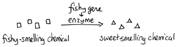 Note that although we show this biochemical pathway as leading from the fishy-smelling chemical to the sweet-smelling chemical in one step, it is likely that there are many other enzymes that act after the fishy enzyme to make the final, sweet-smelling product. In either case, blocking the pathway at the step catalyzed by the fishy enzyme would explain the fishy smell.
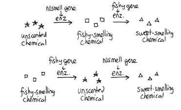 Alternatively, nosmell may not be part of the biosynthetic pathway for the sweet smelling chemical at all. It is possible that the normal function of this gene is to transport the sweet-smelling chemical into the cells from which it is released into the air, or maybe it is required for the development of those cells in the first place. It could even be something as general as keeping the plants healthy enough that they have enough energy to do things like produce floral scent.

Optimized(40MB).pdf")


Optimized(40MB).pdf")
Optimized(40MB).pdf")
Optimized(40MB).pdf")
Optimized(40MB).pdf")
Optimized(40MB).pdf")
Optimized(40MB).pdf")
Optimized(40MB).pdf")
Optimized(40MB).pdf")
Optimized(40MB).pdf")
Optimized(40MB).pdf")
Optimized(40MB).pdf")
Optimized(40MB).pdf")
Optimized(40MB).pdf")

Optimized(40MB).pdf")
Optimized(40MB).pdf")
Optimized(40MB).pdf")

Optimized(40MB).pdf")
Optimized(40MB).pdf")
Optimized(40MB).pdf")
Optimized(40MB).pdf")
Optimized(40MB).pdf")


Optimized(40MB).pdf")
Optimized(40MB).pdf")
Optimized(40MB).pdf")
Optimized(40MB).pdf")


/07%3A_Linkage_and_Mapping/7.06%3A__Genetic_Mapping#:~:text=For%20example%2C%20if%20two%20loci,9).&text=The%20genetic%20map%20distance%20is,of%20DNA%20between%20two%20loci.")


.jpg")

/07%3A_Linkage_and_Mapping/7.06%3A__Genetic_Mapping")


Optimized(40MB).pdf")
Optimized(40MB).pdf")
Optimized(40MB).pdf")
Optimized(40MB).pdf")
Optimized(40MB).pdf")
Optimized(40MB).pdf")

Optimized(40MB).pdf")


.svg)
.svg&oldid=507847250)
_Pressed;_root_meristem_of_Vicia_faba_(cells_in_anaphase,_prophase).jpg)
.svg)
.svg)
.svg)
.jpg)
![DNA animation [gif]](https://commons.wikimedia.org/w/index.php?title=File:DNA_animation.gif&oldid=667176899)