9.6 Experimental Determination of Recombination Frequency
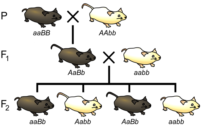
Let us now consider a complete experiment in which our objective is to measure recombination frequency (Figure 9.6.1). We need at least two alleles for each of two genes, and we must know which combinations of alleles were present in the parental gametes. The simplest way to do this is to start with pure-breeding lines with contrasting alleles at two loci. For example, we could cross short-tailed (aa), brown mice (BB) with long-tailed (AA), white mice (bb). Thus, (aaBB) are short-tailed and brown, while (AAbb) are long-tailed and white (Figure 9.6.1 P cross). Based on the genotypes of the parents, we know that the parental gametes will be aB or Ab (but not ab or AB), and all the progeny will be dihybrids, AaBb. We do not know at this point whether the two loci are on different chromosomes, or whether they are on the same chromosome, and if so, how close they are to each other.

The recombination events that may be detected will occur during meiosis in the dihybrid individual. If the loci are completely or partially linked, then prior to meiosis, alleles aB will be located on one chromosome, and alleles Ab will be on the other chromosome. These are the parental gametes based on our knowledge of the genotypes of the gametes that produced the dihybrid. Thus, recombinant gametes produced by the dihybrid will have the genotypes ab or AB.
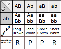
Now that we have identified the parental and recombinant gametes, how do we determine the genotype of the gametes produced by the dihybrid individual? The most practical method is to use a test cross (Figure 9.6.1 F1 to tester), in other words, to mate AaBb to an individual with only recessive alleles at both loci (aabb). This will give a different phenotype in the second generation for each of the four possible combinations of alleles in the gametes of the dihybrid (Figure 9.6.2).

We can then infer unambiguously the genotype of the gametes produced by the dihybrid individual, and therefore calculate the recombination frequency between these two loci. For example, if only two phenotypic classes were observed in the F2 (i.e., short tails and brown fur (aaBb), and white fur with long tails (Aabb), we would know that the only gametes produced following meiosis of the dihybrid individual were of the parental type: aB and Ab, and the recombination frequency would therefore be 0%. Alternatively, we may observe multiple classes of phenotypes in the F2 in ratios, as shown in Table 9.6.1.
| Tail Phenotype | Fur Phenotype | Number of Progeny | Gamete from Dihybrid | Genotype of F2 from Test Cross | (P)arental or (R)ecombinant |
|---|---|---|---|---|---|
| Short | Brown | 48 | aB | aaBb | P |
| Long | White | 42 | Ab | Aabb | P |
| Short | White | 13 | ab | aabb | R |
| Long | Brown | 17 | AB | AaBb | R |
Given the data in Table 9.6.1, the calculation of recombination frequency is straightforward:
[latex]\begin{align}\text{RF}&=\frac{\text{# recombinant offspring}}{\text{Total offspring}}\\\text{RF}&=\frac{13+17}{48+42+13+17}\\&=0.25\end{align}[/latex]
Because the recombination frequency is below 0.30, we can say that the tail length gene and the fur colour gene are partially linked.
Note: The use of linkage and recombination frequency will be extended to Genetic Mapping in Chapter 11.
Media Attributions
- Figure 9.6.1 Original modified by Deyholos (2017), CC BY-NC 3.0, Open Genetics Lectures
- Figure 9.6.2 Original by Canham (2017), CC BY-NC 3.0, Open Genetics Lectures
References
Canham, L. (2017). Figure 9. Punnett Square of example test cross…[digital image]. In Locke, J., Harrington, M., Canham, L. and Min Ku Kang (Eds.), Open Genetics Lectures, Fall 2017 (Chapter 18, p. 7). Dataverse/ BCcampus. http://solr.bccampus.ca:8001/bcc/file/7a7b00f9-fb56-4c49-81a9-cfa3ad80e6d8/1/OpenGeneticsLectures_Fall2017.pdf
Deyholos, M. (2017). Figure 8. An experiment to measure recombination frequency…[digital image]. In Locke, J., Harrington, M., Canham, L. and Min Ku Kang (Eds.), Open Genetics Lectures, Fall 2017 (Chapter 18, p. 7). Dataverse/ BCcampus. http://solr.bccampus.ca:8001/bcc/file/7a7b00f9-fb56-4c49-81a9-cfa3ad80e6d8/1/OpenGeneticsLectures_Fall2017.pdf
Media Attributions
- Figure 9.6.1 Punnett square showing Parental, F1 and F2 generations, to show the production of recombinant progeny, which allows the researcher to measure recombination frequency between two partially-linked loci. The traits being investigated here are coat colour and tail length. [Back to Figure 9.6.1]
- Figure 9.6.2 A Punnett square shows an example of a test cross. The homozygous recessive tester organism can only produce one gamete type, so only one is listed. Phenotypes are listed below each genotype. Using the phenotypes and what we know of the parents, we can identify which phenotypes came from recombinant or parental gametes. [Back to Figure 9.6.2]

